

You are using an out of date browser. It may not display this or other websites correctly.
You should upgrade or use an alternative browser.
You should upgrade or use an alternative browser.
Excel help please.
- Thread starter Colbaker
- Start date
More options
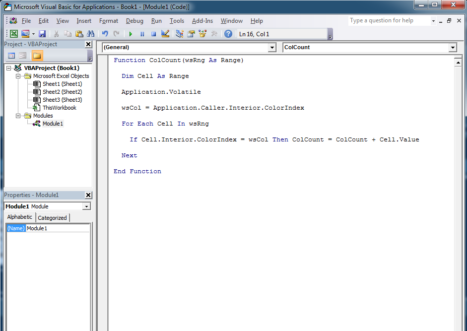
View all postsOk, the following function (formula) will sum the cells in a range that are the same colour as the cell you put the function in.
Function ColCount(wsRng As Range)
Dim Cell As Range
Application.Volatile
wsCol = Application.Caller.Interior.ColorIndex
For Each Cell In wsRng
If Cell.Interior.ColorIndex = wsCol Then ColCount = ColCount + Cell.Value
Next
End Function
-To use it, open the VBA window in the workbook you want to use this in.
-Right click the Workbook in the Project Explorer (the left hand window in the VBA editor) and Insert a module.
-Double click the module
-Paste the code above into the right hand bit of the window (as per screenshot below)
You can now use =ColCount(Your range) as a formula like you would SUM.
The function counts the cells in a range that are the same colour as the cell it is put in.
So if you want to sum Orange cells, write the formula in a cell and then colour that cell orange.
Wow OK thanks for that, I really gotta learn me some VBA, still messing with the basics of normal excel.
Thanks for this though much appreciated.
Im starting to get the hang of this now, It's strange what a good feeling writing a formula that works gives me.
I still haven't got the hang of nesting one formula inside another, What i am trying to do is count the amount of YES's in A1 - A8 and then if it has Yes on that line i need to do an equation working out if the proceeding 2 Cells which have numbers in them take less time.
So for instance Cell A1 has Yes, Cell B1 has the number 22 and Cell C1 has the number 30, on sheet 2 i want the equation to search the YES table for the amount of Yes's then when it has that number work out how many of the Yes lines have the 3rd cell as a larger number than the 2nd.
Does that make any sense?
Once again all, thanks for the reply's, i don't think i explained it well, i think i will explain exactly what i am trying to do, This is sheet 1..

and this is sheet 2

M/O/L stand for More, On Time, Less and equates to time taken in the estimates time and actual time, so F2 has the letter L in it because the actual time taken was less the estimated time. This is not done by an equation though, What would this equation be, something like
=IF(D2>E2,"L","M",if(D2=E2,"O","")), Although that doesnt work, The first bit says if the number in E2 is greater than D2 then it puts and L in, if not then it puts an M in, on the second bit if(D2=E2,"O","")) im trying to say if D2 and E2 are the same then put an O in but that doesnt work, Any ideas on this one?
Also on sheet 2 i have done this equation =COUNTIF(Sheet1!C2:C8,"Bottle") for #job packed which effectively searches for the word bottle and counts it, In C2 what i want to do is put the amount of "BOTTLE" jobs were packed on time and then i can repeat that for the amount of bottle jobs not on time and early, I have tried a few ways of trying to nest IF with Countif but cannot seem to get them to work. Any idea's?
Thanks guys.
There is a way to populate the 2nd table without doing that first though.
I'll just put the kid to bed and then teach you array formulas!
Array formulas sound interesting, Strangely enough i am just putting my boys to bed.
Will keep checking

Ok thanks that worked.
Still don't really understand what the -- part actually does, could you try to explain in lamens terms please.
Also is there any rules when nesting a formula when it comes to comma's and brackets? the reason i ask is i notice some have multiple brackets, does a formula always go in chronological order?
Many thanks for the brilliant reply's.
I am going to have another read tomorrow to see if the info clicks as i have a feeling my brain switched itself off about 3 hours ago as it is just not sinking in.
thats what happens when i work 13 hours then try to learn some excel formula's when i get home
I am going to have another read tomorrow to see if the info clicks as i have a feeling my brain switched itself off about 3 hours ago as it is just not sinking in.
thats what happens when i work 13 hours then try to learn some excel formula's when i get home
Once again all, thanks for the reply's, i don't think i explained it well, i think i will explain exactly what i am trying to do, This is sheet 1..
and this is sheet 2
M/O/L stand for More, On Time, Less and equates to time taken in the estimates time and actual time, so F2 has the letter L in it because the actual time taken was less the estimated time. This is not done by an equation though, What would this equation be, something like
=IF(D2>E2,"L","M",if(D2=E2,"O","")), Although that doesnt work, The first bit says if the number in E2 is greater than D2 then it puts and L in, if not then it puts an M in, on the second bit if(D2=E2,"O","")) im trying to say if D2 and E2 are the same then put an O in but that doesnt work, Any ideas on this one?
Also on sheet 2 i have done this equation =COUNTIF(Sheet1!C2:C8,"Bottle") for #job packed which effectively searches for the word bottle and counts it, In C2 what i want to do is put the amount of "BOTTLE" jobs were packed on time and then i can repeat that for the amount of bottle jobs not on time and early, I have tried a few ways of trying to nest IF with Countif but cannot seem to get them to work. Any idea's?
Thanks guys.
Could i do a SUMPRODUCT equation that still firstly searches for the word Vial, Bottle..etc but instead of working out the actual and estimated times, Looks into Sheet 1 column F and counts the amount of Bottle that has the Letter "O" in the F column.
Something like =SUMPRODUCT(--(Sheet1!$E$2:$E$8=Sheet2!$A2),--(Sheet1!$H:$H="O"))
or mayeb =SUMPRODUCT(Sheet1!$E$2:$E$8=Sheet2!$A2, COUNTIF(Sheet1!H2:H23,"O"))
Although neither of those work maybe it shows you more what i am looking for.
Last edited:
Woooo Hooooo, I think i got it..
=SUMPRODUCT((Sheet1!E:E=A2)*(Sheet1!H:H="O"))
I was not times the amount of the specific word i.e Vial with the amount of "O", Simple really.
Good feeling when you come up with an equation all by yourself, couldn't have done it without you guys though
=SUMPRODUCT((Sheet1!E:E=A2)*(Sheet1!H:H="O"))
I was not times the amount of the specific word i.e Vial with the amount of "O", Simple really.
Good feeling when you come up with an equation all by yourself, couldn't have done it without you guys though
Ok new one i am grappling with at the moment, See below

What i am trying to do is, lets say in the JOHN working box (the one with the border) i want an equation that checks today date (F2) then looksup the corresponding date in the day and date chart, then if on that date John has a Y i want the equation to auto put in Y or if it is an N i was the cell to auto put in an N.
I am sure it is some sort of VLOOKUP with maybe an nested IF, but cant seem to get anything to work.
Any idea's?
ah that actually makes sense ,
The funny thing is i was doing that but in the date section i did the =today() sum and it would obviously never work because it didnt go up to that date in column B, that's what i get for trying to do it whilst my 2 year old is running around.
See below..

How would i use 2 variable's, so i want to enter a name in WHO's WORK DAY then in the IS HE WORKING cell i want it so say either Y or N using the data from the left section.
Once again thanks for all your help.
, The funny thing is i was doing that but in the date section i did the =today() sum and it would obviously never work because it didnt go up to that date in column B, that's what i get for trying to do it whilst my 2 year old is running around.
See below..

How would i use 2 variable's, so i want to enter a name in WHO's WORK DAY then in the IS HE WORKING cell i want it so say either Y or N using the data from the left section.
Once again thanks for all your help.
OK Thanks that worked on my first instance, So in order to try and understand i changed the parameters a little to use get data from another sheet...see below..
sheet 1 (BRANCH INFO)

sheet 2 ROTA

Now i though this should be simple enough as not much actual parameters have changed, on BRANCH INFO sheet in F8 (WORKING) i did this..
=INDIRECT("R"&MATCH(F1,ROTA!B2:B70,0)+1&"C"&MATCH(F5,ROTA!C1:E1,0 )+2,0)
It only ever comes up with a 0 and i cannot see why, i think i have given the equation all the correct parameters as i understood it.
Any idea's what im doing wrong?
Its because you haven't told it to look on the Rota sheet. I haven't tested this as I'm on my phone but try putting 'rota'! or rota! in front of the R, but still within the speech marks.
Ah ok, this just goes to show I don't really understand the R and C parts, I will give it a go in the morning and let you know but still really want to understand what exactly is happening, maybe tomorrow with a fresh brain it might click.
Thanks Wessimo, That works, I still am unsure why though, Im going to have to look into this further, I don't even know CONCATENATE so will look into that first and then maybe it will explain what the R and C actually do and why putting ROTA! next to R worked.
This is advanced stuff but i do find i learn faster being thrown in at the deep end
This is advanced stuff but i do find i learn faster being thrown in at the deep end
Im afraid i need some help again please.
In order to learn Excel in my currently very busy lifestyle (Children off school and very busy 48 hour weeks) i have effectively created a company in which i need to create spreadsheets for, sort of giving myself problems to solve. I am coming on well considering (many thanks to some tutoring from Wessimo) but have got stuck on this little issue.
Anyway, see below..

What i have done above is created a Data mine in order to use the below table to get some info from, The names at the top starting from cell C1 are the employee's, The column that says BRANCH give codes for each branch (easier than doing address's), there is also a column for AREA, There are multiple Branches in each Area. (i hope i have explained that)

Ok, On the above page on the spreadsheet i were i want to filter the data using a formula, The box that covers C2 and 3 as a merged cell is where i want to put enter the data.
What i am trying to get it to do is when i enter the AREA (for instance AREA A) under the B6 column i want it to auto populate each cell with only the Branch numbers that correspond with that area, Vlookup will only produce the first branch, then in the next cells to the relevant branch i want it to add all the names of the people who have FULL ACCESS, PARTIAL and NONE.
Is this even possible, I have tried using the Match formula but i can't get it to do what i want.
Any idea's or if this way seems overly complicated could you recommend a better way for me to filter the people who have Full, Partial or no Access to certain branches within an Area?
I know its a lot to ask and i have really given myself one hell of a task here but i know you guys can help, my google skill haven't helped at all.
In order to learn Excel in my currently very busy lifestyle (Children off school and very busy 48 hour weeks) i have effectively created a company in which i need to create spreadsheets for, sort of giving myself problems to solve. I am coming on well considering (many thanks to some tutoring from Wessimo
) but have got stuck on this little issue.Anyway, see below..

What i have done above is created a Data mine in order to use the below table to get some info from, The names at the top starting from cell C1 are the employee's, The column that says BRANCH give codes for each branch (easier than doing address's), there is also a column for AREA, There are multiple Branches in each Area. (i hope i have explained that
)
Ok, On the above page on the spreadsheet i were i want to filter the data using a formula, The box that covers C2 and 3 as a merged cell is where i want to put enter the data.
What i am trying to get it to do is when i enter the AREA (for instance AREA A) under the B6 column i want it to auto populate each cell with only the Branch numbers that correspond with that area, Vlookup will only produce the first branch, then in the next cells to the relevant branch i want it to add all the names of the people who have FULL ACCESS, PARTIAL and NONE.
Is this even possible, I have tried using the Match formula but i can't get it to do what i want.
Any idea's or if this way seems overly complicated could you recommend a better way for me to filter the people who have Full, Partial or no Access to certain branches within an Area?
I know its a lot to ask and i have really given myself one hell of a task here but i know you guys can help, my google skill haven't helped at all.
I'm not sure I follow you completely but it sounds like a pivot table would be a good starting point
Tried a pivot table but couldn't get it to do what i want.
Yeah, that's possible, I have something similar set up in a spreadsheet i did at work a couple of weeks ago.
It'd be easier if you could send me the spreadsheet to work on though and then i'll explain it.
edit:
It is possible but you're making it really complicated, i'm halfway there but beginning to wonder how to explain all the functions i'm using!
You'd be better of restructuring the way the data is stored in the first place.
Is the "data mine" based on something in real life or just how you envisioned it coming out the database or whatever you hold that information in?
In my fictional company we have multiple employee's who cover the whole of the south east, they need access to all branches in each area but i am trying to make a quick search report that shows who has what access (i.e Colin has partial access to U111 in Area E and full access to all other branches in AREA E), Im not sure if i have set out the Data correctly, I cant help feeling i have over complicated a simple solution.
I could send you the spreadsheet if it would make it a little easier?
Thanks for your help. nothing like throwing myself in at the deep end