

You are using an out of date browser. It may not display this or other websites correctly.
You should upgrade or use an alternative browser.
You should upgrade or use an alternative browser.
Excel help please.
- Thread starter Colbaker
- Start date
More options
Thread starter's postsAs above, you can write a custom function in VBA so you can use it like SUMIF, i wrote one years ago for someone at work if you need any help?
The only other option is to use SUBTOTAL on a filtered list if you're on Excel 2010 (maybe 2007 i can't remember) where you can filter on colours.
The only other option is to use SUBTOTAL on a filtered list if you're on Excel 2010 (maybe 2007 i can't remember) where you can filter on colours.
Soldato
- Joined
- 19 Dec 2006
- Posts
- 9,262
- Location
- Saudi Arabia né Donegal
How are you determining cell colour at the moment? Is it possible to use that in the equation?
How are you determining cell colour at the moment? Is it possible to use that in the equation?
Good point, i assumed the OP meant he had manually coloured the cells, if it's conditional formatting then there may be a way to do it with formulas.
Ok, the following function (formula) will sum the cells in a range that are the same colour as the cell you put the function in.
Function ColCount(wsRng As Range)
Dim Cell As Range
Application.Volatile
wsCol = Application.Caller.Interior.ColorIndex
For Each Cell In wsRng
If Cell.Interior.ColorIndex = wsCol Then ColCount = ColCount + Cell.Value
Next
End Function
-To use it, open the VBA window in the workbook you want to use this in.
-Right click the Workbook in the Project Explorer (the left hand window in the VBA editor) and Insert a module.
-Double click the module
-Paste the code above into the right hand bit of the window (as per screenshot below)
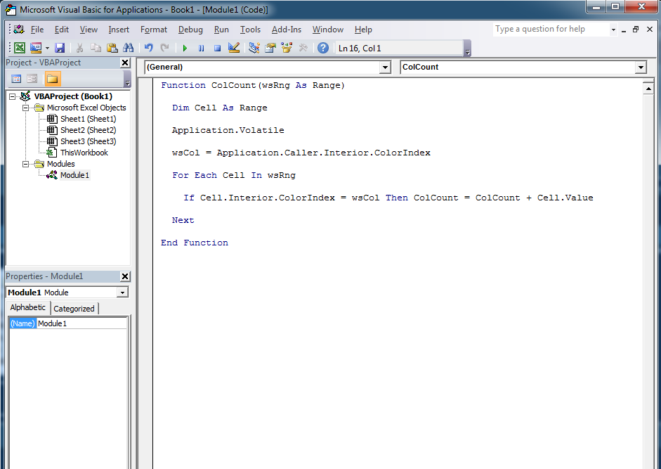
You can now use =ColCount(Your range) as a formula like you would SUM.
The function counts the cells in a range that are the same colour as the cell it is put in.
So if you want to sum Orange cells, write the formula in a cell and then colour that cell orange.
Function ColCount(wsRng As Range)
Dim Cell As Range
Application.Volatile
wsCol = Application.Caller.Interior.ColorIndex
For Each Cell In wsRng
If Cell.Interior.ColorIndex = wsCol Then ColCount = ColCount + Cell.Value
Next
End Function
-To use it, open the VBA window in the workbook you want to use this in.
-Right click the Workbook in the Project Explorer (the left hand window in the VBA editor) and Insert a module.
-Double click the module
-Paste the code above into the right hand bit of the window (as per screenshot below)
You can now use =ColCount(Your range) as a formula like you would SUM.
The function counts the cells in a range that are the same colour as the cell it is put in.
So if you want to sum Orange cells, write the formula in a cell and then colour that cell orange.
Ok, the following function (formula) will sum the cells in a range that are the same colour as the cell you put the function in.
Function ColCount(wsRng As Range)
Dim Cell As Range
Application.Volatile
wsCol = Application.Caller.Interior.ColorIndex
For Each Cell In wsRng
If Cell.Interior.ColorIndex = wsCol Then ColCount = ColCount + Cell.Value
Next
End Function
-To use it, open the VBA window in the workbook you want to use this in.
-Right click the Workbook in the Project Explorer (the left hand window in the VBA editor) and Insert a module.
-Double click the module
-Paste the code above into the right hand bit of the window (as per screenshot below)
You can now use =ColCount(Your range) as a formula like you would SUM.
The function counts the cells in a range that are the same colour as the cell it is put in.
So if you want to sum Orange cells, write the formula in a cell and then colour that cell orange.
Wow OK thanks for that, I really gotta learn me some VBA, still messing with the basics of normal excel.
Thanks for this though much appreciated.
Im starting to get the hang of this now, It's strange what a good feeling writing a formula that works gives me.
I still haven't got the hang of nesting one formula inside another, What i am trying to do is count the amount of YES's in A1 - A8 and then if it has Yes on that line i need to do an equation working out if the proceeding 2 Cells which have numbers in them take less time.
So for instance Cell A1 has Yes, Cell B1 has the number 22 and Cell C1 has the number 30, on sheet 2 i want the equation to search the YES table for the amount of Yes's then when it has that number work out how many of the Yes lines have the 3rd cell as a larger number than the 2nd.
Does that make any sense?
So you want to nest if functions.
An if formula is basically
=(Your Criteria, Output if true, Output if false)
So you would start by looking for the Yes Values
=if(A1="Yes","True","False")
Then instead of saying true if it find yes, you want to add another criteria.
=if(A1="Yes",if(C1>B1,"True","False"))
So if your first criteria is true it moves on to fined the second.
You could also use the AND function to specify two criteria that need to both be met.
=IF(AND(A1="Yes",C1>B1),"True","False")
Last edited:
Once again all, thanks for the reply's, i don't think i explained it well, i think i will explain exactly what i am trying to do, This is sheet 1..

and this is sheet 2

M/O/L stand for More, On Time, Less and equates to time taken in the estimates time and actual time, so F2 has the letter L in it because the actual time taken was less the estimated time. This is not done by an equation though, What would this equation be, something like
=IF(D2>E2,"L","M",if(D2=E2,"O","")), Although that doesnt work, The first bit says if the number in E2 is greater than D2 then it puts and L in, if not then it puts an M in, on the second bit if(D2=E2,"O","")) im trying to say if D2 and E2 are the same then put an O in but that doesnt work, Any ideas on this one?
Also on sheet 2 i have done this equation =COUNTIF(Sheet1!C2:C8,"Bottle") for #job packed which effectively searches for the word bottle and counts it, In C2 what i want to do is put the amount of "BOTTLE" jobs were packed on time and then i can repeat that for the amount of bottle jobs not on time and early, I have tried a few ways of trying to nest IF with Countif but cannot seem to get them to work. Any idea's?
Thanks guys.
There is a way to populate the 2nd table without doing that first though.
I'll just put the kid to bed and then teach you array formulas!
Array formulas sound interesting, Strangely enough i am just putting my boys to bed.
Will keep checking

In fact you don't even need array formulas....
There is a function called SUMPRODUCT that when you enter 2 columns, will multiply each row and then total the results, i.e.
A B A x B
1 2 2
2 3 6
3 4 12
4 5 20
5 6 30
Total 70
=SUMPRODUCT(COLUMNA, COLUMNB) will give you 70 without having to multiply each row out and then sum them.
You can then also use another function that will check for conditions and force Excel to return a 1 or 0 for the row depending if it is true or false.
So if you want to check column C for the type of vessel, and then whether the Estimated Time is the same as the Actual time you can do the following.
=SUMPRODUCT(--(Sheet1!$C$2:$C$8="Bottle"),--(Sheet1!$D$2:$D$8=Sheet1!$E$2:$E$8))
It's the "--" in front of the brackets that's important, it tells Excel to check the condition and then return 1 or 0, so in the first part it's checking the vessel you have in column C to see if it is bottle, if it is it will put a 1 in that position, the second is checking whether the Est and Actual time are the same, again putting a 1 in place if they are.
So basically it ends up doing the following in the background, A is the is it bottle check, B is checking the on time.
A B A x B
0 0 0
0 0 0
0 0 0
0 0 0
1 0 0
1 1 1
0 0 0
Total 1
You can also get rid of the hard coded "Bottle" by referring to the cell that has the word in it.
If you type this =SUMPRODUCT(--(Sheet1!$C$2:$C$8=Sheet2!$A2),--(Sheet1!$D$2:$D$8=Sheet1!$E$2:$E$8)) into cell C2 of Sheet 2, you can then drag it down into cells C3 and C4, and then across into cells D2 and E2, in D2 and E2 change the "=" in the second part of the sumproduct to either "<" or ">" and then drag those down, the whole table will populate with the totals.
Reading back that's a lot of stuff, if it doesn't make sense let me know.
Ok thanks that worked.
Still don't really understand what the -- part actually does, could you try to explain in lamens terms please.
Also is there any rules when nesting a formula when it comes to comma's and brackets? the reason i ask is i notice some have multiple brackets, does a formula always go in chronological order?
The "--" basically tells Excel that whatever is between the brackets that immediately follow it needs to be "resolved" into True (1) or False (0).
i.e. it checks every cell in the range for the condition, in the example above it checks C2:C8 and sees if they contain the value "Bottle".
So with the data you were using, 2 cells contain "Bottle", so Excel resolves that range to a series of 1s and 0s.
Is it Bottle?
0
0
0
0
1
1
0
The second checks if D2 = E2, D3 = E3 etc and resolves that into a series of 1s and 0s
Is it on Time
0
0
1
0
0
1
0
The SUMPRODUCT then multiplies those two sets of data by each other and totals the results.
A x B = AB
0 x 0= 0
0 x 0= 0
0 x 1= 0
0 x 0= 0
1 x 0= 0
1 x 1= 1
0 x 0= 0
Total = 1 row where the vessel is a bottle and the Actual = Estimate
I'll have to try and think how to explain the brackets thing, but basically yes, it works left to right, you open the brackets when you start a function and then close the function with a bracket you'll always have the same amount of "("s as ")"s.
So when you write
=IF(C5>D5,"L",IF(C5<D5,"M","O"))
The first "(" opens the first IF statement, there is another IF statement nested within that which is where the 2nd "(" is, and then both IF statement are closed with the "))".
The reason it is 2 brackets together at the end is that both the IFs end there, it could look like this written another way...
=IF(C5<>D5,IF(C5>D5,"M","L"),"O")