Excel help please.

Many thanks for the brilliant reply's.

I am going to have another read tomorrow to see if the info clicks as i have a feeling my brain switched itself off about 3 hours ago as it is just not sinking in.

thats what happens when i work 13 hours then try to learn some excel formula's when i get home :D
 
Once again all, thanks for the reply's, i don't think i explained it well, i think i will explain exactly what i am trying to do, This is sheet 1..
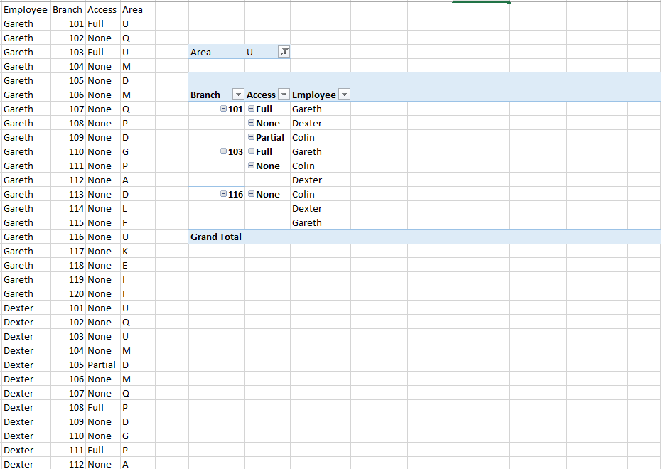


and this is sheet 2


M/O/L stand for More, On Time, Less and equates to time taken in the estimates time and actual time, so F2 has the letter L in it because the actual time taken was less the estimated time. This is not done by an equation though, What would this equation be, something like

=IF(D2>E2,"L","M",if(D2=E2,"O","")), Although that doesnt work, The first bit says if the number in E2 is greater than D2 then it puts and L in, if not then it puts an M in, on the second bit if(D2=E2,"O","")) im trying to say if D2 and E2 are the same then put an O in but that doesnt work, Any ideas on this one?

Also on sheet 2 i have done this equation =COUNTIF(Sheet1!C2:C8,"Bottle") for #job packed which effectively searches for the word bottle and counts it, In C2 what i want to do is put the amount of "BOTTLE" jobs were packed on time and then i can repeat that for the amount of bottle jobs not on time and early, I have tried a few ways of trying to nest IF with Countif but cannot seem to get them to work. Any idea's?

Thanks guys.

Could i do a SUMPRODUCT equation that still firstly searches for the word Vial, Bottle..etc but instead of working out the actual and estimated times, Looks into Sheet 1 column F and counts the amount of Bottle that has the Letter "O" in the F column.

Something like =SUMPRODUCT(--(Sheet1!$E$2:$E$8=Sheet2!$A2),--(Sheet1!$H:$H="O"))

or mayeb =SUMPRODUCT(Sheet1!$E$2:$E$8=Sheet2!$A2, COUNTIF(Sheet1!H2:H23,"O"))


Although neither of those work maybe it shows you more what i am looking for.
 
Last edited:
Woooo Hooooo, I think i got it..

=SUMPRODUCT((Sheet1!E:E=A2)*(Sheet1!H:H="O"))

I was not times the amount of the specific word i.e Vial with the amount of "O", Simple really.

Good feeling when you come up with an equation all by yourself, couldn't have done it without you guys though :D
 
:D Good going!

Just FYI, the reason =SUMPRODUCT(Sheet1!$E$2:$E$8=Sheet2!$A2, COUNTIF(Sheet1!H2:H23,"O")) didn't work is that you hadn't put ="O" plus, i think, because the ranges weren't the same size, you'd defined rows 2:8 in the first bit and then the entire of column E in the second bit, which confuses Excel. And the COUNTIF was probably used incorrectly.

In the equation you did yourself you'd matched them up by using entire columns in both sides.

Just on that point, if you've got a hefty PC and not much data / formulas that will be fine, sometimes though, bearing in mind i used to build 50MB spreadsheets with links all over the place and massively complicated formulas, not limiting the ranges can impact performance.

Often, if i want to provide contingency for data to be added to the ranges i'm referring to, i still won't use an entire column reference, but perhaps say 10,000 rows.

But honestly, even after 15 years of working with Excel i still learn stuff all the time and get a buzz from doing something new, you're doing well to be using the formulas and taking the flaky lessons we're providing onboard, i've had analysts work for me who couldn't have derived that sumproduct you did after much 1:1 coaching.
 
Last edited:
Ok new one i am grappling with at the moment, See below


What i am trying to do is, lets say in the JOHN working box (the one with the border) i want an equation that checks today date (F2) then looksup the corresponding date in the day and date chart, then if on that date John has a Y i want the equation to auto put in Y or if it is an N i was the cell to auto put in an N.

I am sure it is some sort of VLOOKUP with maybe an nested IF, but cant seem to get anything to work.

Any idea's?
 
Put the Values 2,3 and 4 in cells G4 to I4

Then in G6

=vlookup($F$2,$B$2:$E$18,G$4,0)

=vlookup(what you're looking up, where you're looking it up, which column to return, Must be an exact match)

By putting the 2,3 and 4 above the names you can make the vlookup draggable.

So when you type it into John's cell, it will return the column number in G4, the 2nd column, when you drag it across it will automatically adjust to pick up Pete's column, column 3, etc.
 
ah that actually makes sense :D,

The funny thing is i was doing that but in the date section i did the =today() sum and it would obviously never work because it didnt go up to that date in column B, that's what i get for trying to do it whilst my 2 year old is running around.

See below..


How would i use 2 variable's, so i want to enter a name in WHO's WORK DAY then in the IS HE WORKING cell i want it so say either Y or N using the data from the left section.

Once again thanks for all your help.
 
Put the date as 03/01/2013 and then John as the name, then my example will make sense

=INDIRECT("R"&MATCH(F2,B2:B18,0)+1&"C"&MATCH(H10,C1:E1,0)+2,0)

OK...

The &s in the formula CONCATENATE the various bits in bold into a single string.

So they create a string of

"R" and the result of the Match formula then "C" and then the result of the second Match formula.

The Match formula returns the position of the thing you are looking up in the range you are looking it up in.

The first match will tell you how many rows down the date is in the range (3rd), and then we add 1 to account for the title of the column = 4.

The second match will tell you which column the name is in the list of names (1st), we add 2 to account for the 2 cells to the left of the names = 3

The result of the concatenation is therefore "R4C3"

INDIRECT tells Excel we are going to give it a cell reference as a text string, which is the result of that bit in bold or "R4C3". The ",0" after the bold bit tells Excel that we are giving it the cell reference in what is called the R1C1 style, so it knows it's looking for the 4th row down (R4) and the 3rd column across (C3).
 
OK Thanks that worked on my first instance, So in order to try and understand i changed the parameters a little to use get data from another sheet...see below..

sheet 1 (BRANCH INFO)


sheet 2 ROTA


Now i though this should be simple enough as not much actual parameters have changed, on BRANCH INFO sheet in F8 (WORKING) i did this..

=INDIRECT("R"&MATCH(F1,ROTA!B2:B70,0)+1&"C"&MATCH(F5,ROTA!C1:E1,0 )+2,0)

It only ever comes up with a 0 and i cannot see why, i think i have given the equation all the correct parameters as i understood it.

Any idea's what im doing wrong?
 
Its because you haven't told it to look on the Rota sheet. I haven't tested this as I'm on my phone but try putting 'rota'! or rota! in front of the R, but still within the speech marks.
 
Its because you haven't told it to look on the Rota sheet. I haven't tested this as I'm on my phone but try putting 'rota'! or rota! in front of the R, but still within the speech marks.

Ah ok, this just goes to show I don't really understand the R and C parts, I will give it a go in the morning and let you know but still really want to understand what exactly is happening, maybe tomorrow with a fresh brain it might click.
 
Sorry i hadn't explained it well.

In the original example everything was happening on one sheet, so we didn't have to tell Excel which sheet the data we wanted was in, it just assumes it's in the sheet the formula is written in.

In your second example you were trying to get data from another sheet, but hadn't told Excel that, so it was looking at the cell in row 4 (R4) column 5 (C5) in the sheet the formula was written in (Branch Info), which is blank, which is why Excel brought back a 0 rather than an error such as #N/A or #Ref!, the formula "worked" but was looking at the wrong place.

Therefore if you tell Excel that the data about people working or not is in the Rota Sheet in Row 4 and Column 5 it will find the correct information.

=INDIRECT("'Rota!'R"&MATCH(F1,ROTA!B2:B70,0)+1&"C"&MATCH( F5,ROTA!C1:E1,0 )+2,0)

Imagine it like this if you like.

If you give a courier a package with just a number on it, he assumes it has to be delivered to the same same street as you are giving him the package.

If it is a different street, you have to tell him which street.

This also follows on, if it was a different town (completely different workbook), you'd have to tell him or he just assumes it's the same town as you are giving him the package.
 
Thanks Wessimo, That works, I still am unsure why though, Im going to have to look into this further, I don't even know CONCATENATE so will look into that first and then maybe it will explain what the R and C actually do and why putting ROTA! next to R worked.

This is advanced stuff but i do find i learn faster being thrown in at the deep end :D
 
CONCATENATE is just a function that joins text together.

Yes, by including it in this formula it is getting quite advanced so let's take a step back to understand that first.

If you type your first name into cell A1 and your surname into B1, you would have what would be quite a common extract from a database.

But say you needed your full name in one cell for some reason, you could CONCATENATE the 2 cells to get it.

So in cell C1 you would type =(A1 & " " & B1)

This takes the text in A1, appends a space (" ") and then appends the text in A2.

Note that where you are asking it to pull a value from a cell you just put the cell you want, but where you want to add specific text (in this case a space) you have to put it in speech marks.
 
Im afraid i need some help again please.

In order to learn Excel in my currently very busy lifestyle (Children off school and very busy 48 hour weeks) i have effectively created a company in which i need to create spreadsheets for, sort of giving myself problems to solve. I am coming on well considering (many thanks to some tutoring from Wessimo :D) but have got stuck on this little issue.

Anyway, see below..


What i have done above is created a Data mine in order to use the below table to get some info from, The names at the top starting from cell C1 are the employee's, The column that says BRANCH give codes for each branch (easier than doing address's), there is also a column for AREA, There are multiple Branches in each Area. (i hope i have explained that :D)


Ok, On the above page on the spreadsheet i were i want to filter the data using a formula, The box that covers C2 and 3 as a merged cell is where i want to put enter the data.

What i am trying to get it to do is when i enter the AREA (for instance AREA A) under the B6 column i want it to auto populate each cell with only the Branch numbers that correspond with that area, Vlookup will only produce the first branch, then in the next cells to the relevant branch i want it to add all the names of the people who have FULL ACCESS, PARTIAL and NONE.

Is this even possible, I have tried using the Match formula but i can't get it to do what i want.

Any idea's or if this way seems overly complicated could you recommend a better way for me to filter the people who have Full, Partial or no Access to certain branches within an Area?

I know its a lot to ask and i have really given myself one hell of a task here but i know you guys can help, my google skill haven't helped at all.
 
Yeah, that's possible, I have something similar set up in a spreadsheet i did at work a couple of weeks ago.

It'd be easier if you could send me the spreadsheet to work on though and then i'll explain it.

edit:

It is possible but you're making it really complicated, i'm halfway there but beginning to wonder how to explain all the functions i'm using!

You'd be better of restructuring the way the data is stored in the first place.

Is the "data mine" based on something in real life or just how you envisioned it coming out the database or whatever you hold that information in?
 
Last edited:
Yeah, that's possible, I have something similar set up in a spreadsheet i did at work a couple of weeks ago.

It'd be easier if you could send me the spreadsheet to work on though and then i'll explain it.

edit:

It is possible but you're making it really complicated, i'm halfway there but beginning to wonder how to explain all the functions i'm using!

You'd be better of restructuring the way the data is stored in the first place.

Is the "data mine" based on something in real life or just how you envisioned it coming out the database or whatever you hold that information in?

In my fictional company we have multiple employee's who cover the whole of the south east, they need access to all branches in each area but i am trying to make a quick search report that shows who has what access (i.e Colin has partial access to U111 in Area E and full access to all other branches in AREA E), Im not sure if i have set out the Data correctly, I cant help feeling i have over complicated a simple solution.

I could send you the spreadsheet if it would make it a little easier?

Thanks for your help. nothing like throwing myself in at the deep end :D
 
You'd be far better setting the data up differently.

I'd have 4 columns for this, Employee, Area, Branch, Access

Then, as ArchAngel says, a pivot table would do the job really quickly.

Pivot_zps62ec6ebd.png
 
Back
Top Bottom