Excel help!

Man of Honour
Joined
5 Jun 2003
Posts
91,741
Location
Falling...
I wonder if you can help me... I'm having a blonde moment today (I blame the stag do last weekend, and weeks of getting to work for 7am... long days) and the fact I'm not used to Office 2010 yet.

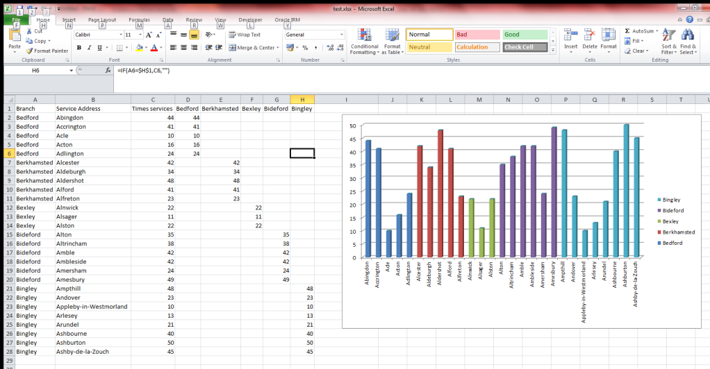
I've got the follow data:

Column1 Column2 Colum3
Site Name Count


I've plotted the name vs count (column2 along the x axis and column3 along the y axis). That's fine.

However, I cannot for the life of me remember how to add column1 so that it colour codes each bar of the chart. I want to identify on the bar chart/legend different colours for different column1 data but use the column2 data vs column3.

So basically I want column2 vs column3 to remain as it is, but just colour code using column1 the bar chart...

Does that make any sense? :o

Help :o
 
Not quite sure what you're asking - do you just want column 1 to be a different colour on the chart to 2 & 3?

Go into the series options and select the data for the first column as series 1, then make series 2 the rest of the data, you'll then be able to change the colour and type of chart of these independently (actually you can probably manually do it anyway by just clicking the actual bar, then clicking again so only the bar you want is selected before right clicking for option to colour change)
 
It's confusing to explain.

I have over 50 entries in column 1,2 &3

Column 1 contains the branch name
Column 2 contains the address that the branch services
Column 3 contains the number of times column 2 (address) is serviced.

I have plotted column 3 along the y axis and column 2 along the X axis.

I want to identify the bar chart points by colour code as to which branch does which address without adding any extra columns on the sheet without having to edit each data value and colour coding it individually/manually. Does that clear it up? (Probably not!)
 
Last edited:
Does the same address repeat? Or are they all different and you want x number of different coloured bars? That would look.....interesting

Assuming there are multiple hits on the same address quickest way I can think of would be to stick a filter on the table, filter for that address and make that series 1- do the same again for series 2-x then you can colour code that bar for each branch that services the same address.
 
Can't quite fathom what exactly you're trying to do I'm afraid. But you can auto change colours using Conditional Formatting, which includes Data Bars and Colour scales; This is under Home - Conditional Formatting on the ribbon at the top.
 
Sounds like you need to use "Conditional Formatting". Any chance of a screenshot to show us exactly what you're looking at?
 
I take it you are looking for something like this?
excel.png


The trick is to lay the data out with the address on the left, the branch on the top, and the number of visits entered at the point the two intersect.

In the example above, I've used a simple "If statement" to transfer the data from coloumn format to table format. When I've created the graph, I've started by selecting column B and C. Them I right clicked on the graph and hit select data, and manually moved the data selector from C to D:H.

Hope that helps.
 
Spot on. Thank you.

I didnt even think about changing the layout of the data.

Thanks to everyone for enduring my rubbish explanations
 
Back
Top Bottom